曲面模型建構
![]()
![]()
![]()
在草圖、Part Studio 中提供此功能
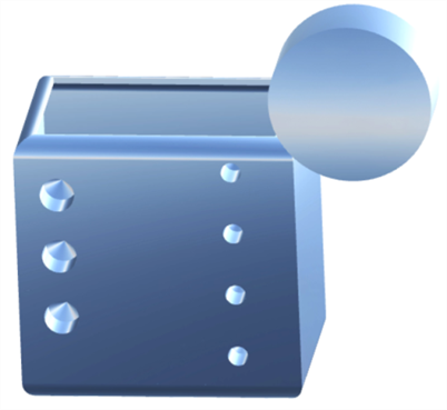
曲面是零件外部的單邊呈現,並沒有質量或厚度。
曲面模型建構此一模型建構方式可讓設計人員建立實體建模工具無法單獨產生的複雜幾何特徵和有機形狀。與實體模型建構相比,曲面模型建構更適用於自由的形狀和特徵。
例如,一個實心立方體可以被分成六個不同的面。每個面代表一個包圍實體體積的曲面,從而形成立方體。曲面建模可讓您將立方體的每個面建構成一個單獨的曲面。在建立了立方體的六個邊之後,將曲面都加在一起,從而建立一個封閉的體積來形成實體零件。
曲面幾何可用來:
-
建立實體零件:
-
使用「加厚」特徵來將曲面加厚以形成實體零件。
-
使用「封閉」特徵,形成一個封閉的體積來建立實體零件,其中每條邊線都與兩個面相連。
-
-
建立幾何建構線 (模具的分模線、將幾何混合與橋接在一起、支援疊層拉伸與填補以配對曲率和相切)。
-
使用更複雜的幾何取代實體面 (使用「替換面」特徵)。
曲線和曲面連續性測量的是兩條曲線或兩個曲面連接處的平滑度。在建構曲線與曲面以建立幾何模型時,若要產生最流暢或連續的有機形狀,連續性變得至關重要。
G (或幾何) 標識是用來決定曲線/曲面的連續性 (G0 到 G3)。在 Onshape 中,這些標識與許多曲線和曲面特徵中的 "配對" 選項相關聯 (例如,橋接曲線、圓角、面混合與其他等等)。這些連續性的分類及其定義概述如下:
-
G0 (配對位置) - 配對 2 個曲線/曲面間的位置。兩個曲線/曲面會在接合處共享相同的位置。
-
G1 (配對相切) - 配對 2 個曲線/曲面間的相切。兩個曲線/曲面相接觸並共享一個到兩端相等的共同角度。圓角是此類連續性配對的一個很好範例。
-
G2 (配對曲率) - 配對 2 個曲線/曲面間的曲率 (半徑)。兩個曲線/曲面相接觸且相切,並在相接處有相同的曲率 (兩者有相同的半徑)。
-
G3 (配對流動) - 配對 2 個曲線/曲面間的流動。兩個曲線/曲面相接觸且相切,會有類似的曲率,並顯示曲率在其長度方向上的變化量 (流動)。
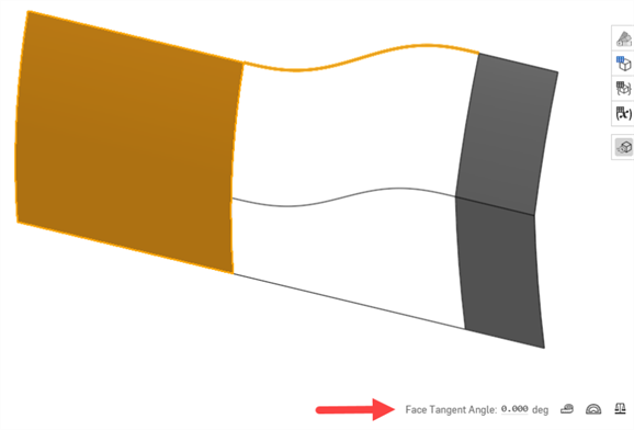
使用橋接曲線特徵,您可以建立兩條曲線間的一條橋接曲線 (下方以橘色顯示) ,然後將其開始與結束位置、相切性、曲率以及流動配對 (或是兩者的某種組合;例如,在開始處「配對位置」,在結束處「配對曲率」):
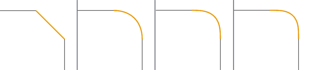
從左到右:G0 (配對位置)、G1 (配對相切)、G2 (配對曲率)、 G3 (配對流動)
將此延伸到曲線之外,您可以在 2 個曲面間建立一個曲面,然後以相同的方式配對其開始與結束的連續性:
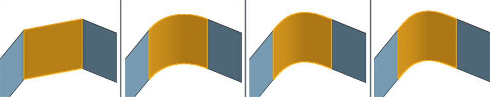
從左到右:G0 (配對位置)、G1 (配對相切)、G2 (配對曲率)、 G3 (配對流動)
當使用曲線/曲面分析工具來分析曲線或曲面的連續性時,您可以看到隨著每個連續性配對的進展,曲線/曲面間的連接變得更為平滑,並顯示更平滑的曲率梳。無法使用曲線/曲面分析來分析 G0 (配對位置) ,因為直線並沒有曲率。
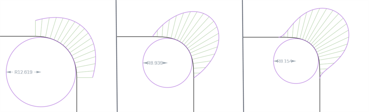
從左到右:G1 (配對相切)、G2 (配對曲率)、 G3 (配對流動)
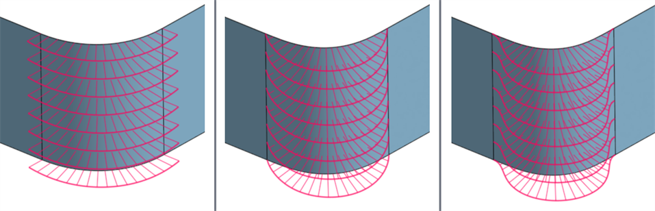
從左到右:G1 (配對相切)、G2 (配對曲率)、 G3 (配對流動)
當使用斑馬條紋工具來分析曲線或曲面的連續性時,隨著每個連續性配對的進展,曲線/曲面間的連接變得更為平滑。 當您從 G0 (配對位置) 上升至 G2 (配對連續) 時,曲面邊上的斑馬條紋變得越來越平滑:
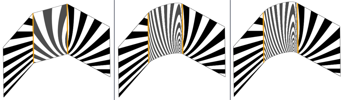
從左到右:G0 (無連續性)、G1 (配對相切)、G2 (配對曲率)、與 G2 (配對曲率)
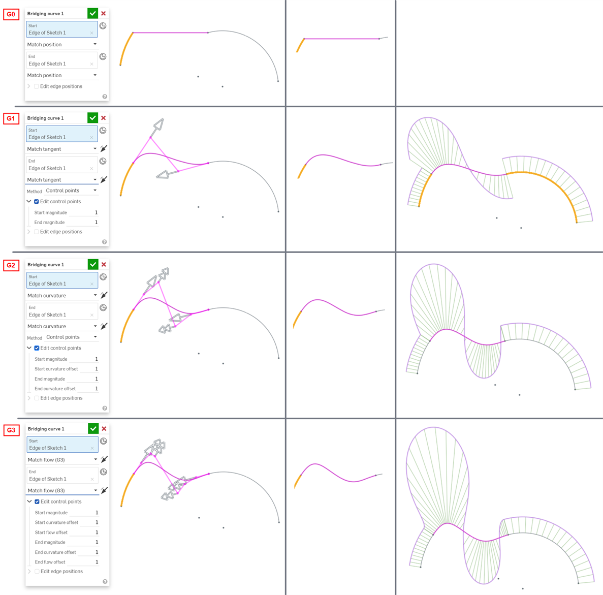
下方的範例說明在兩條非線性曲線間的橋接曲線的連續性。橋接曲線是以紫紅色來表示的。第一欄中顯示「橋接曲線」對話方塊,以及連續性的選擇與結果 (啟用了「編輯控制點」),中間欄顯示停用了「編輯控制點」的橋接曲線 ,最後的欄位顯示對所有曲線的曲線/曲面分析:
在您模型中為曲線和曲面連接的連續性選擇完全取決於在每個交會處/邊線所需的連續性等級。並沒有正確或是錯誤的曲面連續性。
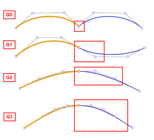
此外,較高階的連續性需要更多的控制點來達成。G0 僅需要一個控制點 (端點),G1 需要兩個,G2 需要三個,G3 則需要四個。兩端均受 G3 限制的貝茲曲線至少需要八個控制點,每端四個。
使用曲面建模需要額外的步驟才能建立高品質的曲面。這些步驟會增加效能,避免瑕疵,以及簡化複雜曲面的生成。
-
曲線/曲面分析 - 視覺檢視與分析在 Part Studio 中草圖的曲率。透過按一下 Shift+c,在草圖、零件或曲面上按右鍵,或是點按介面右下角的「顯示分析工具」圖示 (
 ) 來存取「曲線/曲面分析」對話方塊。
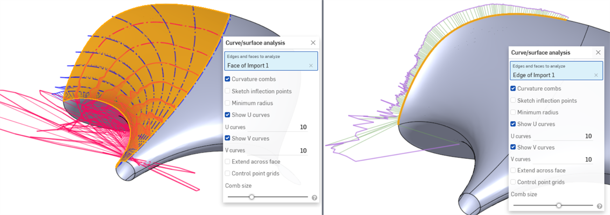
這些工具會顯示曲率梳形 (沿邊線或面在某一點的曲率強度),以及控制點網格。在理想情況下,曲率梳形的曲率應該逐漸增加或減少。
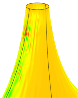
下方範例在沒有評估工具的情況下看起來不錯,但在啟用了曲率/曲面分析時,顯示了極大的曲率波動 (特別是在下方左圖的紅色 U 方向上)。外側邊線尤其有問題 (下方右圖):
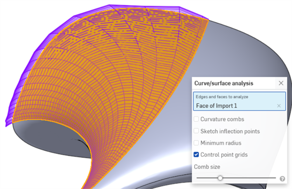
此外,控制點網格是測量曲面複雜度的方式。控制點的流動和密度可以顯示模型中有太多的控制點:
-
連接分析 - 存取或報告在 Part Studio 或草圖中曲線與曲面間的連接。從介面右下角的「顯示分析工具」圖示 (
) 來存取「連接分析」對話方塊。選擇要分析的曲線或曲面;在選擇之後對話方塊 (下圖所示) 會自動顯示結果,且在圖形區域中會有色彩對應的指標。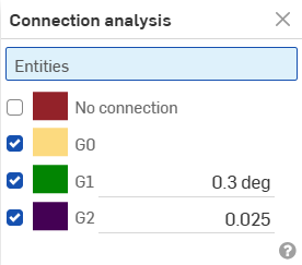
-
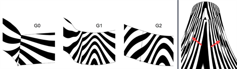
斑馬條紋與色彩對應 - 斑馬條紋代表在 Part Studio 或組合件中目前模型、面或曲面的條紋空間反射。這可以讓您查看橫跨邊線與面的曲率是否是對正及連續的。從介面右下角的「顯示分析工具」圖示 (
) 來存取「斑馬條紋」。斑馬條紋與 G0 或位置連續性不配合。在 G1 或相切連續性中,其在邊線處直接相配,但之後卻急劇分開。在 G2 或曲率連續性中,斑馬條紋平滑地穿過邊線 (下方左圖所示)。斑馬條紋可讓您查看曲面上的缺陷或瑕疵 (下方右圖所示):
-
曲率色彩對應 - 套用您選擇的漸層色彩到 Part Studio 中的面或曲面上以對曲率進行更深入的探查。您可以調整漸層色彩的色階,從不同類型的色彩對應中選擇,以獲得最佳的視覺呈現來辨識曲面連續性與邊線間的轉換。
最常見的色彩對應曲率選項是高斯曲率,對決定曲面曲率是否有局部缺陷或劇烈變化是相當有用的。在上方斑馬條紋影像中偵測到的波紋,於高斯曲率觀察下更為明顯:
-
二面角分析 - 從介面右下角的「顯示分析工具」圖示 (
) 來存取「二面角分析」。這會顯示在共用邊線的 2 個曲面的法線之間的夾角。如果角度是零,這 2 個曲面在沿邊線的該位置至少是相切的。在下方的範例中,二面角刻意地從硬摺痕變化到曲線另一端的平滑相切混合中: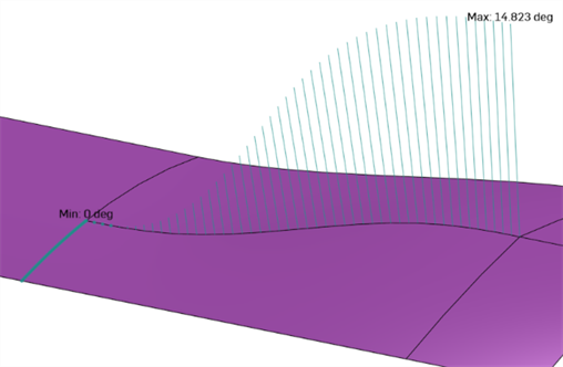
-
偏差分析 - 顯示在草圖或 Part Studio 中 2 條連續曲線間的最小與最大偏差,或是在 Part Studio 的 2 個曲面間的最小與最大偏差。
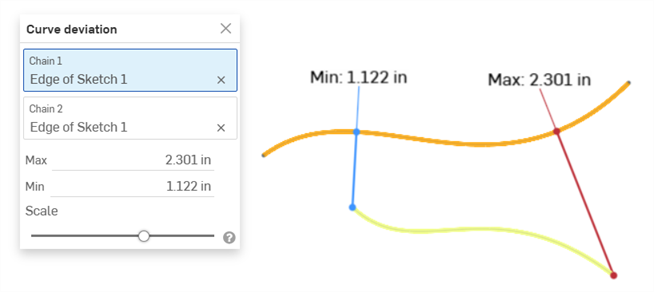
顯示兩條曲線間最大/最小偏差的範例
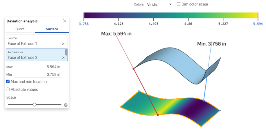
顯示「來源」曲面與「來測量」曲面間最大/最小偏差的範例
詳細資訊請參考偏差分析。
-
反射分析 - 使用您選擇的反射材質和環境影像在圖形區域中渲染模型。
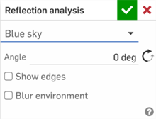
詳細資訊請參考反射分析。
-
強調顯示邊界線 - 以紅色強調顯示任何開放的邊線。可以從「視角立方體 」下方的「攝影機與渲染選項」下拉清單 (
 ) 來存取「強調顯示邊界線」。當你嘗試找出曲面中的開放區域以形成實體時,這非常有用。
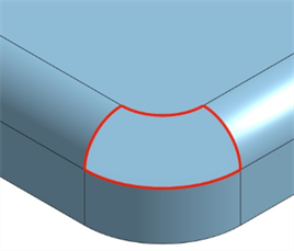
-
面相切角度 - 面相切角度 (一個測量工具) 提供曲線在接近面時是否在其端點與面相切的快速回饋。先選擇面,相切角度會顯示在測量工具的左側。這對在完成 疊層拉伸或邊界曲面之前是測試連續性是相當又用的:
-
以高品質檢視 - 為檢視開啟最高可用的鑲嵌品質,這對於找出曲線缺陷與準確評估連續性至關重要。從「視角立方體」下方的「攝影機與渲染選項」下拉清單 (
) 來存取「以高品質檢視」。 -
帶邊線塗彩/相切邊線 - 有助於更清晰地觀察邊線連續性。從「視角立方體」下方的「攝影機與渲染選項」下拉清單 (
) 來存取這兩個選項。
-
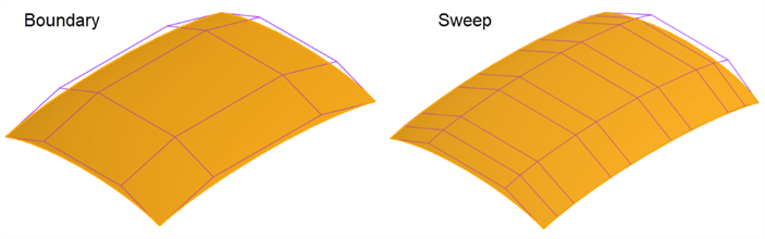
邊界曲面 - 某些特徵對建立曲面的曲線控制不佳,導致曲面過於複雜並降低了曲面的品質。邊界曲面可以完全控制 U 與 V 方向的曲線。產生曲面的複雜程度是僅與所輸入曲線類似的。「疊層拉伸」、「掃掠」與「填補」特徵 會在一或兩個方向上建立無法控制的曲線,使曲面變得複雜。
例如,使用「邊界曲面」與「掃掠」建立同一曲面。「掃掠」會沿著路徑的 V 方向形成曲線,進而產生過於複雜的曲面:
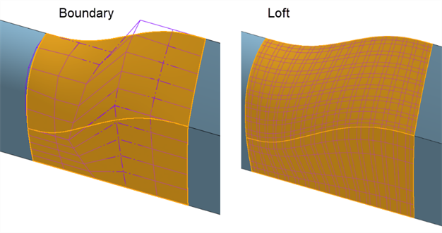
使用「邊界曲面」與「疊層拉伸」來建構同一曲面。「疊層拉伸」會在兩個方向建立密集的控制點網格:
-
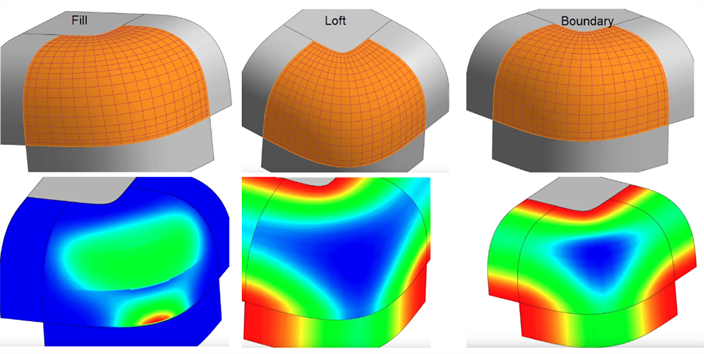
填補 -「填補」會修補曲面上的小孔。在填補之後,評估所產生的曲面以確保曲面的品質。在下方的範例中,「填補」會在底部加入波紋。「疊層拉伸」建立了沒有波紋的較佳控制點網格,但「邊界曲面」建立了最平滑與最最一致的結果:
-
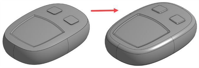
面混合與圓角 -「面混合」與「圓角」會建立類似於投影或分割操作的複雜邊線。由於「面混合」與「圓角」特徵的複雜性,由它們所建立的邊線會更容易失敗並引入缺陷。由於這通常只是外觀上的修飾,所以最好先建構虛擬交角的曲面,最後再加入這些特徵:
-
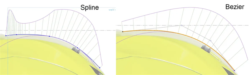
使用貝茲而不是樣條 - 「樣條」有沿著曲線定義的點,並在起點與終點上有控制點。「貝茲」有沿著控制多邊形定義的控制點,多邊形是從曲線偏移而來的。「貝茲」曲線會平滑地增加和減少,連續性不會中斷:
-
將曲線保持簡單 - 使用貝茲工具並從 3 或 4 個控制點 (包括端點) 來開始。加入最少可能數量的樣條點。
-
貝茲的階數等於控制點的數量減 1。貝茲的階數通常應是 3、5、或 7。將單一貝茲曲線的階數限制為 7 是最好的,因為在較高的階數時,數學的計算會變得非常複雜。移動一個控制點會影響整條曲線,較高階數的曲線會難以調整而不引入缺陷。
-
使用一致的控制點流動,以確保平滑的曲率變化,避免意外的強度變更。
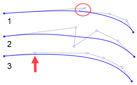
下方是一些控制點位置不佳的曲線範例。第一條曲線在第一與第二個點之間有之字形 (由圓圈框出)。第二條曲線在曲線上方與下方都放置了控制點。只有當您打算為曲線加入轉折點時,才適合改變要在那一邊放置控制點。第三條曲線在控制點之間沒有平滑的間距。點之間的間距較其他點間距明顯的不同 (如下方箭頭所指):
-
-
避免從修剪過的邊線或投影曲線建構 - 由於這些是由修剪操作,或具有許多跨度 (線段結在一起) 的 3 次 (cubic) 樣條投影製成,任何由這種曲線構成的曲面都會更加複雜且不完美。
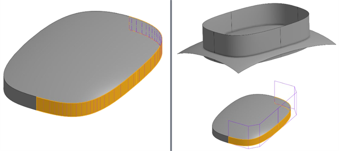
例如,在直接從修剪曲面的邊線建立直紋曲面時,此處的曲面具有更密集的控制點網格 (左下圖)。應改採過度建構兩個曲面,然後使用「相互修剪」來修剪掉相交處的多餘部分 (右下圖):
與其使用投影曲線,可試看看橋接曲線是否可建構出較不複雜的相同幾何。橋接曲線是貝茲曲線,取決於端點條件,可達到 5 的階數。
-
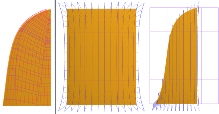
盡量使用四邊曲面 - 四邊曲面有最一致的控制點網格。建立沒有四邊的曲面會導致奇點 (退化) 或不規則間距的控制點 (下圖左側所示)。可過度建構曲面,然後使用「分割」特徵的參考曲面來修剪曲面。這樣可建立具有不同邊線輪廓的曲面,同時保持控制點網格的一致性 (下圖右側所示):
-
盡可能使用對稱 - 為連續性套用限制條件以確保跨中心線的平滑轉換。
-
在草圖中使用有「相切」或「曲率」限制條件的參考線。
-
在 3D 模型中,加入參考曲面以幫助所產生曲面的連續性。
-
-
使用快速鍵功能表與熱鍵 - 使用 shift+c (曲線/曲面分析)、shift+d (二面角分析)、與 shift+r (以高品質檢視)。您也可以在「我的帳戶」>「喜好設定」>「捷徑工具列」 之下自訂捷徑工具列。
這個清單是曲面特徵工具的集合,並非詳盡的清單。在建構曲面時,可能會使用其他的特徵工具。詳細資訊請參考曲面建構。
-
 加厚 - 將厚度加入到曲面上。藉由給予曲面厚度然後將其轉換為實體,在現有零件或曲面上加入或移除材料,或是在路徑上使零件相交來建立新的零件或修改現有的零件。
 -
 封閉 - 選擇可形成實體的空間周圍的所有邊界來建立零件。使用任何互為相交或在邊界相接的曲面組與實體 (包括平面和面) 來建立一個體積。藉由加入或移除零件,或使零件相交來建立新的零件或修改現有的零件。
 -
 圓角 - 選擇「邊線」圓角來圓化尖銳的內部與外側邊線,並定義標準的固定半徑,建立更有造型的圓錐或變化。選擇性地套用「全周」圓角來在兩個對邊間建立一或多個面上無縫的混合。
 -
 面混合 - 圓滑化尖銳的連接或未連接的內部與外部面以建立面之間無縫的混合,或是將混合分離來建立新的面, 並可定義半徑或固定寬度。進一步定義混合的橫截面 (滾動球或掃出輪廓)、對稱、控制、修剪、約束與限制。
 -
 刪除面 - 從零件上移除一個幾何。選擇是否要修復周圍的面 (延伸面直至面相交),為空白加蓋,或將空白保留為開放。如果您沒有零件的參數式歷程記錄時 (通常在匯入的零件中有此狀況),此直接編輯的工具是相當方便的。
 -
 移動面 - 平移、旋轉或偏移一或多個所選的面。如果您沒有零件的參數式歷程記錄時 (通常在匯入的零件中有此狀況),此直接編輯的工具是相當方便的。
 -
 替換面 - 修剪一個面或將面延伸至一新的曲面。如果您沒有零件的參數式歷程記錄時 (通常在匯入的零件中有此狀況),此直接編輯的工具是相當方便的。
 -
 偏移曲面 - 偏移一個現有面、曲面或草圖區域來建立新的曲面。將偏移距離設定為 0 來就地產生一個副本。
 -
 邊界曲面 - 建立或新增由曲面邊界輪廓指定而來的曲面。
 -
 填補 - 定義邊界並使用邊界條件 (而不需使用參考曲面) 來細修曲面以建立一個曲面 (或從曲面建立零件)。
 -
 移動邊界 - 移動曲面的邊界線以延伸或修剪曲面。
 -
 直紋曲面 - 從一條現有邊線、草圖直線或曲線建立一個直紋曲面。
 -
 Mutual trim - Trim two adjacent contiguous sets of surfaces by extending intersections to complete the trim. Each surface set can be flipped to select which side is kept, and all surfaces can be merged into a single surface or unmerged to keep all trimmed surfaces.
 -
 約束曲面 - 從指定公差內的點或網格資料中選擇以建立曲面。顯示偏差並最佳化效能或平滑度。
除了曲面建構工具之外,還可使用曲線來建立曲面的基本建構塊。
這個清單是曲線特徵工具的集合,並非詳盡的清單。在操控曲線時,可能會使用其他的特徵工具。
- 草圖工具 - 草圖工具列中的工具,像是直線、轉角矩形、中心點矩形、中心點畫圓、三點畫圓、切線弧、三點定弧、樣條、點與建構線,可用來建立 Part Studio 中的草圖。
-
 螺旋線 - 使用圓錐或圓柱面、單一軸或結合連接器的 z 軸、或是環狀邊線來建立螺旋線。
 -
 3D 擬合樣條 - 建立穿過連續頂點的 3D 擬合樣條。建立列在零件清單中「曲線」之下的曲線。
 -
 投影曲線 - 建立一條來自兩個草圖投影的曲線 (「兩個草圖」選項),或是建立一條來自曲線投影至面的曲線 (「曲線到面」選項)。
 -
 橋接曲線 - 建立連接任兩個點、頂點或結合連接器的一條曲線。所產生的曲線會列於「特徵」清單與「零件」清單中。
 -
 複合曲線 - 以一條曲線來代表多條邊線。選擇多條相鄰的邊線、草圖圖元、與其他的曲線。選擇非連續的邊線會建立多條的曲線。為每條曲線做出的選擇項目必須在其頂點處交會 (曲線會列於「零件」>「曲線」清單之中)。
 -
 相交曲線 -在兩或多個曲面或面的相交處建立一條曲線。選取的項目必須是相交的。
 -
 修剪曲線 -根據距離修剪或延伸曲線,或是修剪或延伸至邊界圖元。
 -
 等傾線 - 在斜面上建立一條等傾線。等傾線會出現在面相較於其參考定義有某些傾斜的位置。所產生的等傾線會列於「特徵」清單與「零件」清單中。
 -
 偏移曲線 - 藉由在周圍面上偏移邊線來建立與延伸和/或分割新的曲線。
 -
 等參數曲線 - 建立沿面或曲面的 U 方向或 V 方向延伸的平滑曲線。
 -
 編輯曲線 - 選擇草圖圖元或曲線來套用簡化的近似、提高度數、重新定位控制曲線頂點和/或平化至任何 2D 平面來編輯現有的曲線。
 -
 路線曲線 - 建立在 3D 空間中跨越一個或多個平面的多點曲線 (路線路徑)。這對於建立管路路線、配線、以及進階曲面建立中的 NURBS 曲線是非常有用的。
關於曲面建構的更多資源,請造訪我們的學習中心。